Self-diffusion for solving inverse problems
NeurIPS 2025, self-diffusion models, inverse problem, lower level vision, MRI reconstruction
TLDR Self-diffusion solves inverse problems without the need of pretrained generative models via a self-contained iterative process that alternates between noising and denoising steps to progressively refine its estimate of the solution. The full paper is available here and the code is available here.
Abstract Self-diffusion introduces a self-contained iterative process that alternates between noising and denoising steps to progressively refine its estimate of the solution. At each step of self-diffusion, noise is added to the current estimate, and a self-denoiser, which is a single untrained convolutional network randomly initialized from scratch, is continuously trained for certain iterations via a data fidelity loss to predict the solution from the noisy estimate. Essentially, self-diffusion exploits the spectral bias of neural networks and modulates it through a scheduled noise process. Without relying on pretrained score functions or external denoisers on a clean dataset, this approach still remains adaptive to arbitrary forward operators and noisy observations.
Methods To map the estimated noisy solution \(\mathbf{x}_t=\mathbf{x}^{\text{true}}_{t} + \sigma(t) \epsilon_t\) to the true solution \(\mathbf{x}^{\text{true}}\), a self-diffusion process trains a self-denoiser \(D_{\theta_{t,k}}\) at each noise step \(t = T-1, \ldots, 0\) over \(k = 0, \ldots, K-1\) iterations to minimize the loss
\begin{equation} L_{t,k} = | \mathcal{A} D_{\theta_{t,k}}(\mathbf{x}^{\text{true}}_{t} + \sigma(t) \epsilon_t) - \mathbf{y} |^2~, \label{eq:loss} \end{equation}
where \(\mathbf{x}^{\text{true}}_{t}\) is the estimate of \(\mathbf{x}^{\text{true}}\) within noise step \(t\), initialized as \(\mathbf{x}^{\text{true}}_{T} = \epsilon_0\), with \(\epsilon_0 \sim \mathcal{N}(0, I)\). The noise \(\epsilon_t \sim \mathcal{N}(0, I)\) is sampled once at the start of noise timestep \(t\) and is fixed across all \(K\) iterations within that timestep. It is then resampled for the next noise step \(t-1\). The noise schedule is \(\sigma_t = \sqrt{1 - \bar{\alpha}_t},\) where \(\bar{\alpha}_t = \mathop{\textstyle\prod}\nolimits_{i=0}^t (1 - \beta_i)\) and \(\beta_t = \beta_{\text{end}} + \frac{t}{T - 1}(\beta_{\text{start}} - \beta_{\text{end}})\). After \(K\) iterations at each noise step, the self-denoiser \(D_{\theta_{t,k}}\) produce the estimated solution \(\mathbf{x}^{\text{true}}_{t-1}\) for the next noise step \(t-1\). As the noise level \(\sigma(t)\) decreases to zero, the predicted solution converges to the true solution \(\mathbf{x}^{\text{true}}\). Equation \eqref{eq:loss} is expanded into the following form using a first-order Taylor:
\begin{equation} \mathbb{E}_{\epsilon_{t}}[||\mathcal{A}D_{\theta_{t,k}}(\mathbf{x}_t)-\mathbf{y}||^{2}] \approx \underbrace{||\mathcal{A}D_{\theta_{t,k}}(\mathbf{x}_t^\text{true})-\mathbf{y}||^2}_{\text{Data Fidelity Term}} +\underbrace{\sigma(t)^{2}||\mathcal{A}J_D(\mathbf{x}_t^\text{true})||_F^2}_{\text{Regularization Term}}~. \end{equation}
This regularization effect is modulated by the noise level \(\sigma_t\). In early steps of diffusion, where noise is large, the regularization is strong, enforcing smooth outputs and prioritizing low-frequency components. As the process progresses and \(\sigma_t\) decreases, the regularization weakens, allowing the network to focus on finer, high-frequency details. This design leads to an implicit multi-scale learning regime, where the reconstruction transitions from global structure to local refinement. We reveal this process in Fourier space as detailed in the paper.
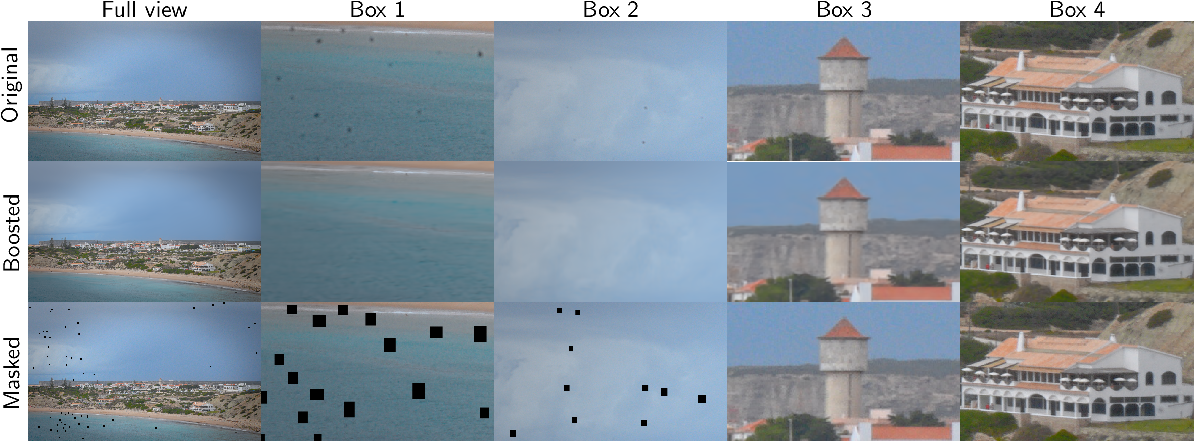
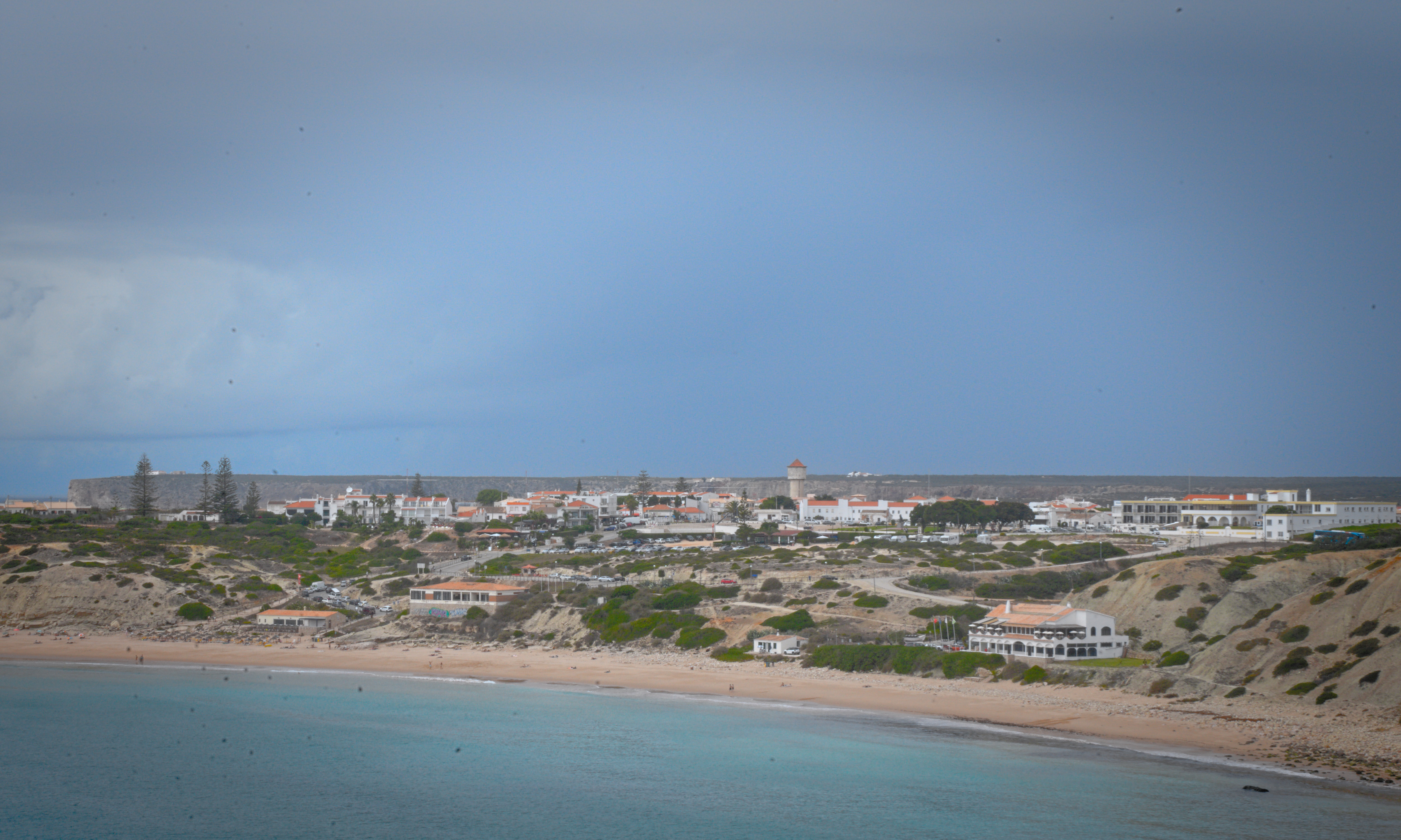
Results As a teaser, we evaluated self-diffusion on a large image of size (5000\(\times\)3000), which is from an inexperienced shooter and corrupted by dust spots and minor noise. We masked the dust spots using a binary mask then restored the image using self-diffusion. Apart from this, we listed some of our results in the paper from different settings such as inpainting, image denoising and MRI reconstruction.


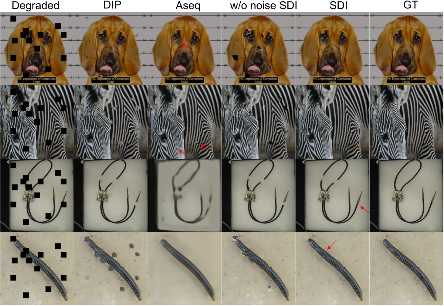
Inpainting: Comparison of inpainting results across different methods (DIP, Aseq, w/o noise SDI, SDI) against the ground truth (GT).

Denoising: Visual comparison of denoising results across different methods against the ground truth. IR-SDE by Luo et al., 2023; FFDNET by Zhang et al., 2018.

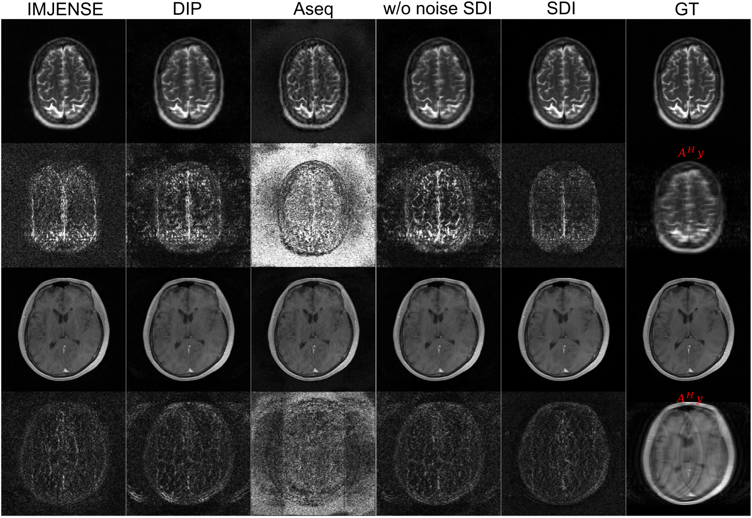
MRI reconstruction: Reconstruction from 4\(\times\) undersampled k-space with 20 ACS lines using different methods (\(\mathcal{A}^H\mathbf{y}\),IMJENSE, DIP, Aseq, w/o noise SDI, SDI) and corresponding error maps are shown.
