Bayesian MRI reconstruction with joint uncertainty estimation using diffusion models

Figure 1. Overview of the proposed method.

Abstract In recent years, the application of deep learning has made significant advancements in fast MRI reconstruction, yielding promising results. However, worries about the uncertainty caused by undersampling strategies and algorithms have limited their usage in clinical practice until now, which could lead to hallucinations. Therefore, the uncertainty assessment constitutes an important step for deep learning-based approaches. The uncertainty is twofold: (1) the uncertainty of weights inside the neural network; and (2) the uncertainty introduced by the missing k-space data points. The uncertainty from missing k-space data points can be addressed in a Bayesian imaging framework.

TLDR All in all, a deep learning-based method has enough capability to generate a realistic-looking image even when the problem is highly underdetermined as a result of undersampling, but the uncertainties inside it cannot be ignored.

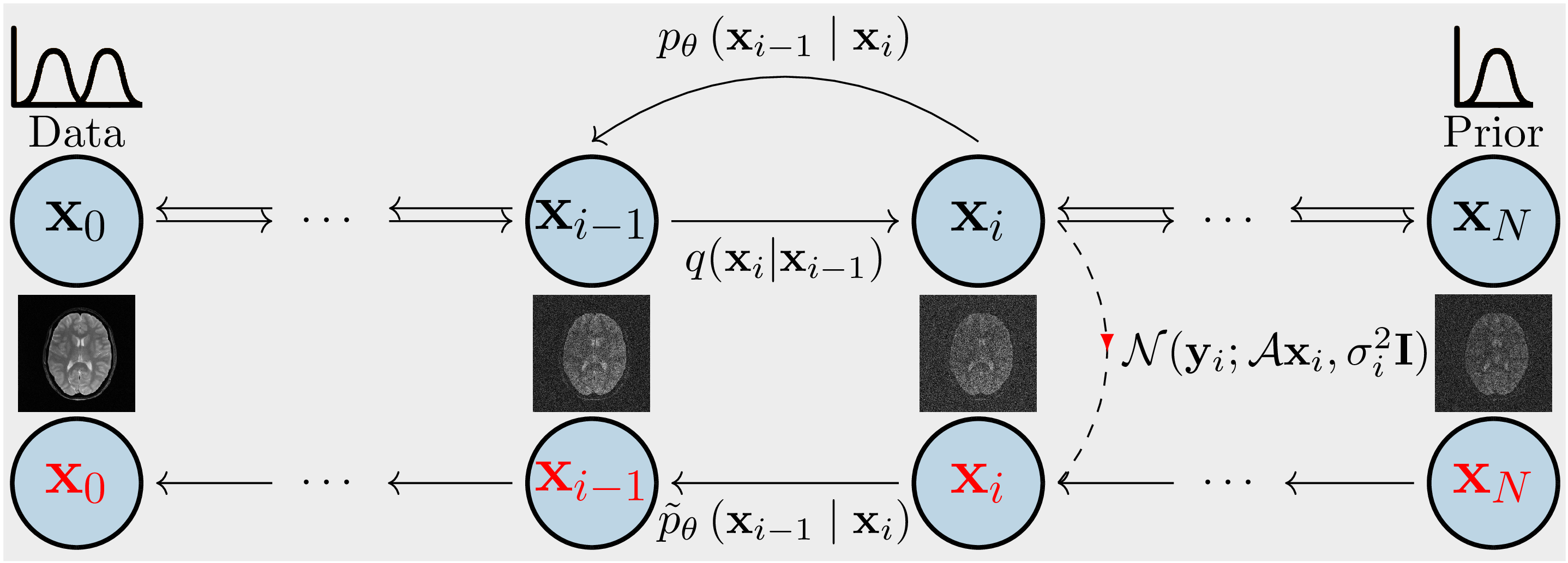
Samples are drawn from the posterior distribution given the k-space using the Markov chain Monte Carlo (MCMC) method. The minimum mean square error (MMSE) and maximum a posterior (MAP) estimates are computed. The chains are the reverse of a diffusion process (c.f., Figure 1). Score-based generative models are used to construct chains and are learned from an image database. The unknown data distribution \(q(x_0)\) of the training images goes through repeated Gaussian diffusion and finally reaches a known Gaussian distribution \(q(x_N)\), and this process is reversed by learned transition kernels \(p_\theta(x_{i-1}|x_i)\). To simulate samples from the posterior of the image given the k-space, \(y\), a new Markov chain is constructed by incorporating the measurement model into the reverse process (red chain).

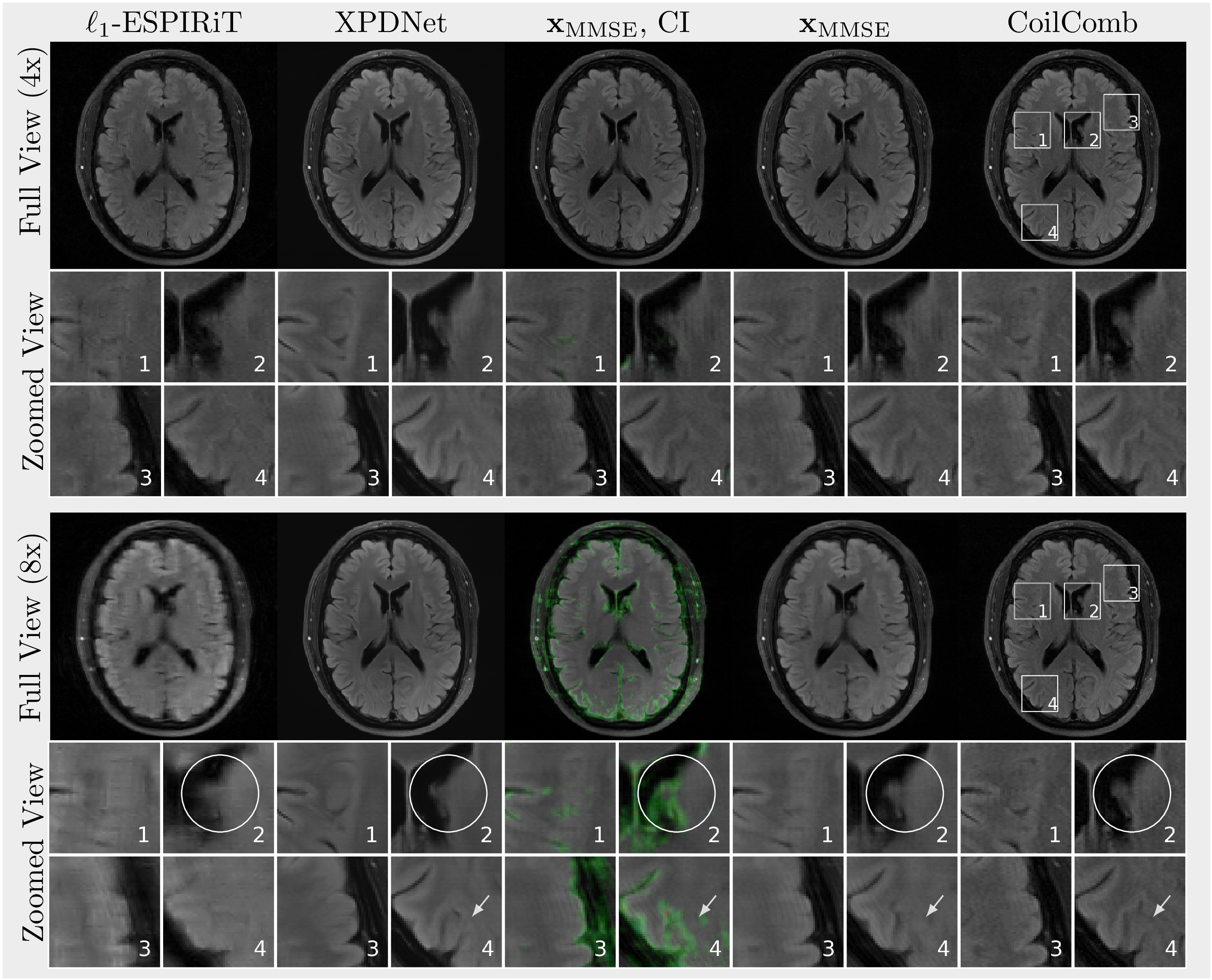
Highlight In Figure 3, reconstructions are \(\ell_1\)-ESPIRiT, XPDNet, \(x_\text{MMSE}\) highlighted with confidence interval (CI), \(x_\text{MMSE}\) and a fully-sampled coil-combined image (CoilComb). All methods provide nearly aliasing-free reconstruction at four- or eightfold acceleration. Hallucinations appear when using 8-fold acceleration and are highlighted with CI after thresholding. Selected regions of interests are presented in a zoomed view.

Figure 3. See if you can find hallucinations above.

Theory Using Bayes’ formula one obtains for each \(i\) the desired distribution \(p\left (x_i \mid y\right )\) from \begin{equation} p\left(x_i \mid y\right) \propto p\left(x_i\right) p\left(y \mid x_i\right)\quad \text{with}\quad p(y|x_i) = \mathcal{CN}\left(y;\mathcal{A} x_i, {\sigma}^2_{\eta} {I}\right), \nonumber \end{equation} where \(\mathcal{A}\) is the parallel MRI forward model, \(x_i\) is the \(i\)-th image and \(y\) is given k-space data (c.f. Figure 1). Starting with the initial density \(q(x_N)\sim \mathcal{CN}(0,I)\) at \(i=N\), one obtains \(p(x_i)\) with transition kernels \(\{p(x_j | x_{j+1})\}_{i \leq j < N}\) \begin{equation} p(x_i) \propto p(x_i | x_{i+1}) \cdot … \cdot p(x_{N-1} | x_N) \cdot q(x_N).\nonumber \end{equation} By estimating the transition kernel with the neural network, one obtains the kernel \(p_\theta(x_i \mid x_{i+1})\) and therefore one can sample \(p_\theta(x_i | y)\) with the unadjusted Langevin Monte Carlo method in order to get an estimate of \(x_i\), i.e. \begin{equation} x_i^{k+1} \leftarrow x_i^{k} + \frac{\gamma}{2}\nabla_{x_i}\log p_\theta(x_{i}^{k}\mid y) + \sqrt{\gamma}{z},\quad z \sim \mathcal{CN}(0, {I}),\nonumber \end{equation} with stepsize \(\gamma > 0\), \(k=1,...,K\) and \(x_i^1 := x^K_{i+1}\) with \(x_N^1 \sim \mathcal{CN}(0, {I})\).

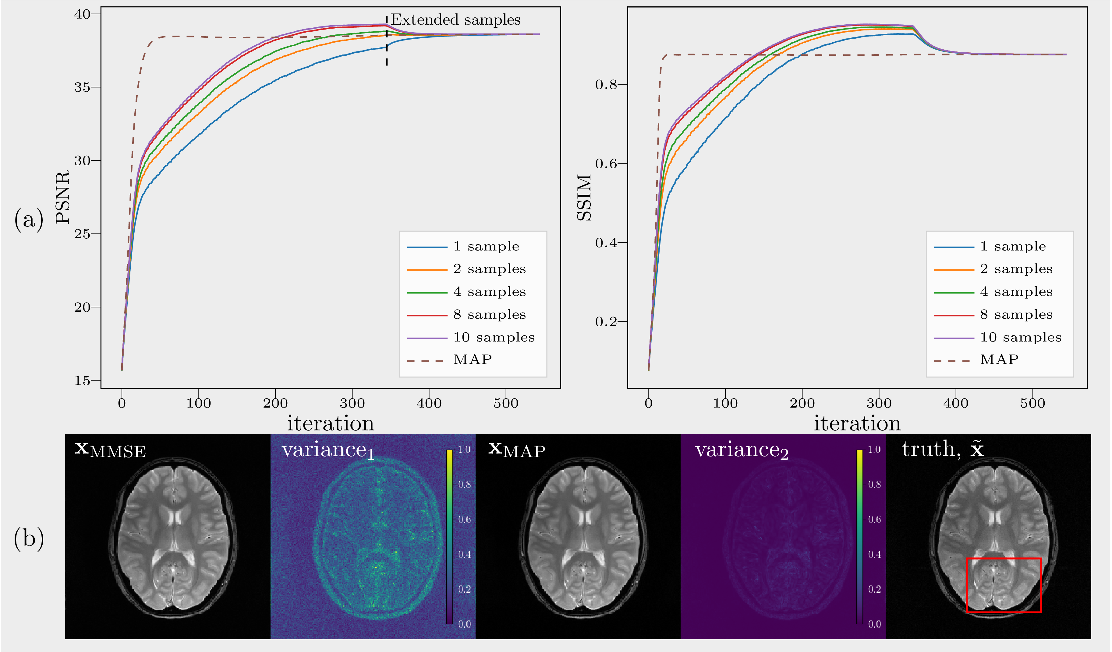
MMSE vs MAP 200 extended iterations after random exploration (i.e, without noise disturbance) and a deterministic estimate of MAP are indicated by solid and dashed lines respectively. (a) PSNR and SSIM over iterations. (b) Variance\(_\text{1}\) and variance\(_\text{2}\) were computed from unextended samples and extended samples respectively. Extended samples converge to \(x_\text{MAP}\).

Figure 4. Have a look at two variance maps.

Conclusion All in all, a deep learning-based method has enough capability to generate a realistic-looking image even when the problem is highly underdetermined as a result of undersampling, but the uncertainties inside it cannot be ignored.