MRI reconstruction using deep Bayesian estimation

Figure 1. Overview of the proposed method.

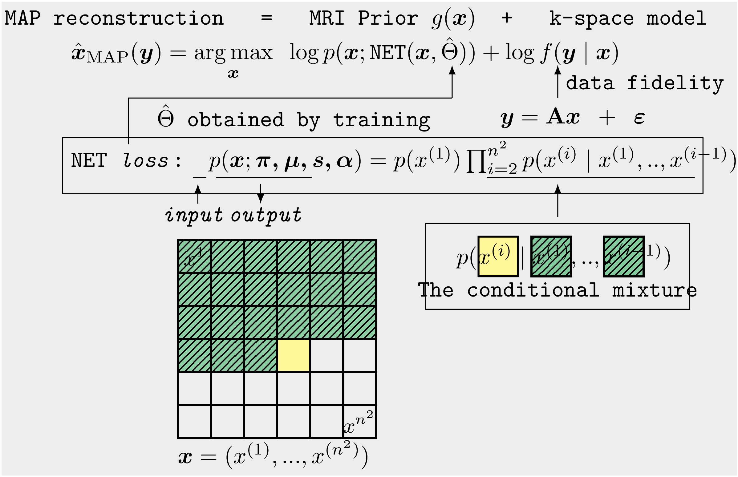
Abstract We developed a deep learning-based Bayesian estimation for MRI reconstruction. The image reconstruction from incomplete k-space measurement was obtained by maximizing the posterior probability (MAP). The autoregressive generative model PixelCNN was utilized as the image prior and the k-space data fidelity was enforced by using an equality constraint. The stochastic back-propagation was utilized to calculate the descent gradient in the process of maximum a posterior, and a projected sub-gradient method was used to impose the equality constraint. In contrast to the other deep learning reconstruction methods, the proposed one used the likelihood of prior as the training loss and the objective function in reconstruction to improve the image quality. In summary, the separation of the image prior and the encoding matrix embedded in the fidelity term made the proposed method more flexible and generic compared with conventional deep learning approaches as shown in Figure 1.

Method There two stages in our approach. The first is to learn prior information from an existing dataset using PixelCNN, and the second is to maximize the posterior using the sub-gradient projection method as illustrated in Figure 2.

With Bayes theorem, one could write the posterior as a product of likelihood and prior: \begin{equation} f(x|y) = \frac{f(y\mid x)g(x)}{f(y)} \propto f(y\mid x )\,g(x ) \label{eq:1} \nonumber \end{equation} where \(f(y\mid x)\) is probability of the measured k-space data \(y\in \mathbb{C}^M\) for a given image \(x\in \mathbb{C}^N\), \(N\) is the number of pixels and \(M\) is the number of measured data points. \(g(x)\) is the prior model that estimates the distribution of MR images. In order to avoid the confusion with the likelihood occurs in modelling the prior, \(f(y\mid x)\) is referred to as k-space likelihood model. The image reconstruction is achieved by exploring the posterior \(f(x\mid y)\) with an appropriate estimator. The maximum a posterior estimation could provide the reconstructed image \(\hat{x}\) that is given by: \begin{equation} {\hat {x }}_{\mathrm {MAP} }(y)={\underset {x}{\operatorname {arg\,max} }}\ f(x \mid y)={\underset {x}{\operatorname {arg\,max} }}\ f(y\mid x)\,g(x)\nonumber \label{eq:2} \end{equation} In this way, the reconstruction problem is recast as posterior probability calculations.

Figure 2. The proposed reconstruction algorithm.

Specifically, we reconstructed images with 256\(\times\)256 matrix size, using the prior model \(g(x)\) that was trained with 128\(\times\)128 images. To reconcile this mismatch, we split one 256\(\times\)256 image into four 128\(\times\)128 patches for applying the prior model. After updating \({s}^{(k+1)}\), four patches for one image were merged to form an image with the original size of 256\(\times\)256. Then the merged image was projected onto \(\{x\mid y = \mathcal{A} x \ + \ \varepsilon\}\). Furthermore, the random shift along phase encoding direction was applied to mitigate the stitching line in-between patches. Figure 3 displays the evolution of image during the process of reconstruction.

Conclusion The Bayesian estimation significantly improved the reconstruction performance, compared with the conventional L\(^1\)-sparsity prior in compressed sensing reconstruction tasks. More importantly, the learnt prior knowledge is generic to many MRI reconstruction scenarios when changing sampling patterns, coils and so on.