The details of flash attention - algorithm
The compuation of self-attention is a key component in transformer models. It is used to compute the attention weights from the query and key vectors and perform the weighted sum of the value vectors. The attention weights are computed using the dot product of the query and key vectors, and then normalized using the softmax function. This step is computationally expensive in terms of both time and memory as it faces memory bound and compute bound issues.
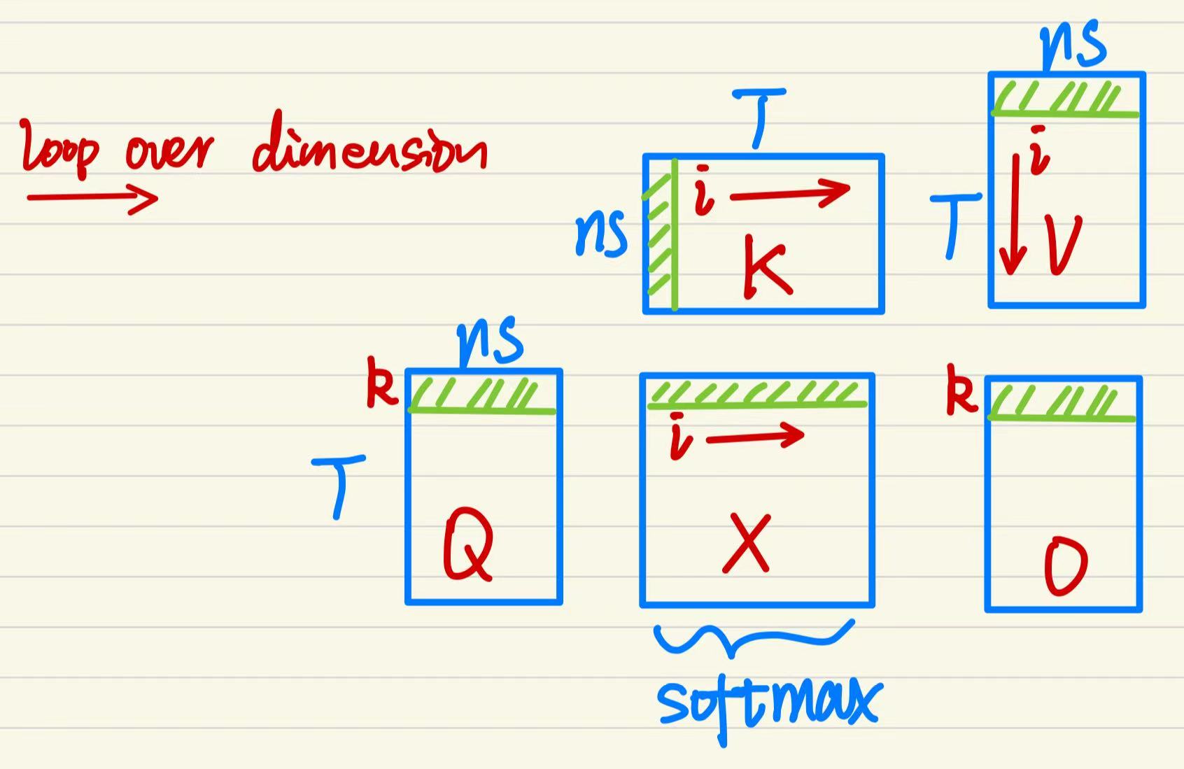
We start with the definition where inputs \(Q, K, V\) typically have shapes \((B, \text{nhead}, N, nd)\). Since batch and head dimensions are independent from attention weights computation, we focus on the sequence length \(N\) and the embedding dimension \(nd\). The illustration below breaks the computation of a single head of self-attention into matrice multiplications. The attention formular is \(\begin{equation} O=\text{Attn}(Q, K, V) = \text{softmax}\left(\frac{QK^T}{\sqrt{d_k}}\right)V~. \end{equation}\) The k-th row of the output matrix is \(\begin{equation} O[k, :]=\sum_{i=1}^N X_s[k, i]\cdot V[i, :]~, \end{equation}\) where \(\begin{align} X_s[k, i]&=\text{softmax}\{i=1:N\vert x_i=X[k,i]=\frac{Q[k, :]K[i, :]^T}{\sqrt{d_k}}\}\\ &=\{i=1:N|\frac{e^{x_i}}{\sum_{j=1}^N e^{x_j}}\}~. \end{align}\)

We cannot simply exponentiate the dot products because \(e^{x_i}\) can easily overflow floating-point limits. To fix this, we use safe softmax. This requires finding the maximum value in the row (\(m_N\)) and subtracting it from every element before exponentiation. Then, this computation involves three distinct steps (loops) over the data:
-
Find the Global Max (\(m_N\)): Iterate through the row to find \(m_N = \max(x_i)\).
-
Compute the Global Sum (\(d_T\)): Iterate again to compute the normalization constant \(d_T = \sum_{i=1}^{N} e^{x_i - m_N}\).
-
Compute the Output: Iterate a third time to calculate the weighted sum \(O[k, :] = \sum_{i=1}^{N} \frac{e^{x_i - m_N}}{d_T} \cdot V[i, :]\).
This approach forces us to separate the calculation into multiple passes. We cannot compute the output until we have finished scanning the entire row to find \(m_N\) and \(d_T\). This requires repeated reading and writing of the \(N \times N\) matrix makes standard attention memory-bounded.
To optimize this, we must ask: Can we merge these main blocks?.
We need a way to calculate the softmax incrementally (online) as we read the data, rather than waiting for the global statistics. This is achieved by maintaining running statistics that update dynamically. Instead of calculating the final max and sum upfront, we define running variables for the \(i\)-th step: 1) the running maximum: \(m_i\); 2) the running sum of exponentials: \(d'_i=\sum_{j=1}^{i} e^{x_j - m_i}\).
Then we have two main steps. In loop 1: \(i=1 \rightarrow N\) when moving from step \(i-1\) to \(i\), we introduce a new value \(x_i\). If \(x_i > m_{i-1}\), our maximum changes. We must rescale our previous accumulations to account for this change.
-
Updating the Max: \(m_i = \max(m_{i-1}, x_i)\)
-
Updating the Sum (\(d'_i\)) by rescaling the previous sum (\(d'_{i-1}\)) by the exponential difference between the old and new max: \(d'_i = d'_{i-1} \cdot e^{m_{i-1} - m_i} + e^{x_i - m_i}\)
Upon reaching the N-th step, we have \(d'_T=d_T\). Then we start loop 2: \(i=1 \rightarrow N\), \(O[k, :] = \sum_{i=1}^{N} \frac{e^{x_i - m_N}}{d'_T} \cdot V[i, :]\)
Can we merge these two loops? Yes, but the second loop is dependent on \(m_N\) and \(d'_T\). Then, we apply the same rescaling logic to the partial output accumulator by defining \(O'_i = \sum_{j=1}^i \frac{e^{x_j - m_i}}{d'_i} \cdot V[j, :]\). As a result, the computation of the output matrix \(O[k, :]\) can be recast into a geometric progression:
\[\begin{align} O'_i &= \sum_{j=1}^i \frac{e^{x_j - m_i}}{d'_i} \cdot V[j, :] \\ & = \sum_{j=1}^{i-1} \frac{e^{x_j - m_i}}{d'_i} \cdot V[j, :] + \frac{e^{x_i - m_i}}{d'_i} \cdot V[j, :] \\ & = \sum_{j=1}^{i-1} \frac{e^{x_j - m_{i-1}}}{d'_{i-1}} \cdot \left( \frac{d'_{i-1}}{e^{x_j - m_{i-1}}} \cdot \frac{e^{x_j - m_i}}{d'_i} \right) \cdot V[j, :] + \frac{e^{x_i - m_i}}{d'_i} \cdot V[i, :] \\ & = O'_{i-1} \cdot \left( \frac{d'_{i-1}}{d'_i} \cdot e^{m_{i-1} - m_i} \right) + \frac{e^{x_i - m_i}}{d'_i} \cdot V[i, :] \end{align}\]Upon reaching the N-th step with these recursive formulas, we have \(O'_T[k, :] = O[k, :]\). By doing this, we can compute the output in a single pass without needing the computation of \(X\) matrix, and write/read it repeatedly to get global max and sum upfront. The next blog post will focus on how to implement this in an efficient way using CUDA.
Enjoy Reading This Article?
Here are some more articles you might like to read next: